Monetary policy makers often face a trade-off between rules based and discretionary policy formulation. While discretionary policy formulation allows flexibility in responding to unexpected shocks, it can simultaneously create uncertainty and reduce credibility. On the other hand, a systematic, rules based approach anchors expectations regarding future monetary policy, helping to stabilize the economy over time. In 1993, the economist John B. Taylor proposed the Taylor rule as a mathematical monetary policy guideline which prescribes how a central bank should set their short term nominal interest rate target in response to inflation deviating from the target inflation rate.

Historical Context

The period between the 1970s and early 1980s was a period of relentless inflation, resulting in stricter monetary policy implementation; for example, when the Federal Funds Rate (the interest rate at which US banks lend funds to each other during a short period) peaking at above 20% in 1981, the resulting aggressive tightening of monetary policy led to a severe recession in the early 1980s, with unemployment in the USA reaching levels over 10% in 1982 (typically around 4%). The crisis resulted in the trust in the Fed’s ability to maintain price stability fading and led to central banks realizing the importance of a systematic monetary policy formulation in anchoring economic expectations, stabilizing the economy and increasing trust in the Fed’s ability to maintain inflation levels low. This monetary instability (in the form of high inflation and unemployment rates) eventually led to the development and adoption of rules based frameworks, such as the Taylor Rule, in regards to monetary policy decisions. It also drove the move towards inflation targeting and the integration of expectations into policy formation models.

The Taylor Rule

The equation Taylor originally proposed was:

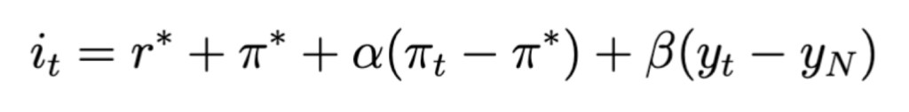
• it is the nominal interest rate

• r∗ is the real interest rate (the nominal interest rate – the inflation rate)

• πt is the current inflation rate

• π∗ is the target inflation rate

• yt is the log of real GDP

• yN the log of potential output (full-employment GDP)

• α, β are weights on the inflation and output gap (0.5 in the original Taylor Rule)

We can apply the Taylor Rule through setting some arbitrary but realistic parameters. Let:

• r∗ = 2%

• π∗ = 2%

• πt = 2% (the target inflation rate)

• yN = 100

• yt = 100 (at potential)

• α, β = 0.5

If we substitute these parameters into the Taylor Rule, we find:

Therefore, we find that when inflation is on target and output is at potential, the Taylor Rule recommends setting the nominal interest rate at 4%.

Calculating the Output Gap

There are various ways in which we can calculate the potential GDP. One of the most commonly used methods is through the use of the Hodrick-Prescott filter which takes the real GDP output of an economy and then smooths the data to separate the long-term trend (potential) from the short-term fluctuations (cycle). Mathematically, the HP filter does this through the following minimization problem:

Where:

• yt is the observed time series

• τt is the unobserved trend component we need to estimate

• λ is the smoothing parameter: a larger λ value results in a smoother trend, making the output less responsive to short-term fluctuations. A smaller λ means the resulting trend follows data more closely

Here, the first summation is in order to fit the minimization problem to the data. The second summation is to smooth the data. From this minimization problem, we derive the Hodrick-Prescott filter:

The Taylor Rule plays a central role in New Keynesian macroeconomic models and Dynamic Stochastic General Equilibrium (DSGE) frameworks, both of which form the backbone of modern monetary policy analysis. In these models, the economy is represented as a system of interrelated economic agents: households, firms and the government, which all make forward looking decisions based on rational expectations. In these contexts, the Taylor Rule provides a systematic and theoretically grounded guideline for setting the nominal interest rate in response to economic conditions, allowing these models to simulate how policy affects output, inflation and expectations over time.

A key concept embedded in the Taylor Rule is the Taylor Principle, which states that a central bank should raise the nominal interest rate by more than one to one with increases in inflation rate (if inflation goes up by 1%, the nominal interest rate should increase by more than 1%). This ensures that real interest rate rises when inflation increases, stabilising prices and preventing runaway inflation. When inflation falls, nominal interest rates decline sufficiently to support demand. Models incorporating the Taylor Principle produce stable equilibriums and are often consistent with observed central bank behaviour over recent decades.

Moreover, the Taylor Rule also enhances credibility and expectations management. As agents in New Keynesian and DSGE models form rational expectations, they anticipate how policy responds to changes in inflation or output. When the central bank follows a transparent, rules-based approach like the Taylor Rule, households and firms can align their wage-setting, investment and pricing decisions with policy objectives. This alignment reduces the need for aggressive interventions, helps anchor inflation expectations and makes inflation targeting more effective.

Overall, the Taylor Rule is not solely a descriptive tool, it is a foundation of modern macroeconomic theory which also links systematic policy, the Taylor principle and rational expectations in order to achieve more stable and predictable outcomes.

Testing empirically 

In order to test how consistently central banks follow the Taylor Rule, or other similar systematic based monetary policy approaches, we need to compare the nominal interest rate set by a central bank and the recommended interest rate from the Taylor Rule.

Plotting the graph comparing the annual effective Federal Funds Rate to the nominal interest rate prescribed by the Taylor Rule, we find the following relationship:

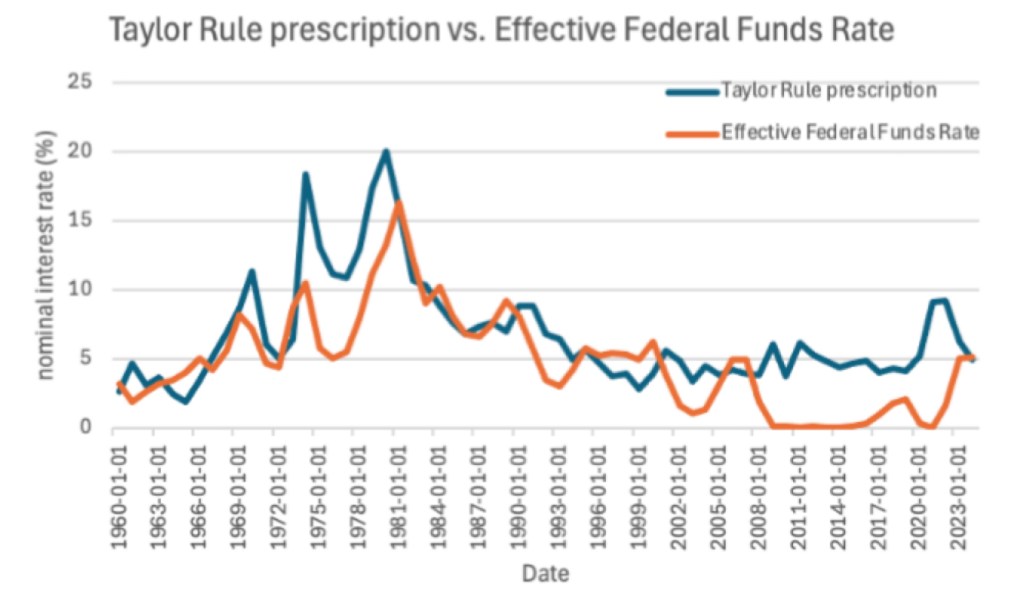
Output gap is calculated as the percentage difference between real GDP and potential GDP. Both the neutral interest rate and target inflation rate are set at 2%.

The graph shows that the Taylor Rule prescription for the nominal interest rate is much more volatile than the effective Federal Funds rate, and often prescribes much more extreme interest rates; for example, in 1975, when the prescribed interest rate was around 18%, and in 1981, when it was 20%. It also highlights the Taylor Rule’s inability to account for macroeconomic variables beyond inflation and the output gap, such as financial instability. For example, during the aftermath of the 2008 financial crisis, the Taylor Rule recommended a nominal interest rate of around 5%, while the effective federal funds rate was 0%, showing the limitations of systematic policy formation frameworks as they fail to capture all aspects of the economy. Despite these deviations, the Taylor Rule generally follows the same trend as the effective Federal Funds Rate consistently in all periods, excluding the period after the 2008 financial crisis, reflecting a potential shift in policy formation frameworks in recent years. Significant deviations are often observed during periods of economic stress, such as post 2008, and after the Covid pandemic, highlighting the limitations of systematic policy formation frameworks.

Criticisms and limitations

However, despite the benefits it offers, there are various limitations regarding the rule’s implementation as well as many critiques of the rule itself. Firstly, the Taylor Rule requires estimates of key unobserved variables such as the neutral interest rate (R2) and the target inflation rate (π∗). In reality, these values are unknown and are therefore often estimates that can change over time due to structural shifts in the economy; for example, the Federal Reserve’s median estimate of the neutral rate is currently between 2.4% and 3.8%. This estimate is already rather vague; however, when we account for the fact that private estimates often differ, for example Vanguard estimates the current neutral interest rate to be lower, at around 1.5%, and other Fed models set it closer to 0.5%, making the rule’s reliability limited due to potential measurement errors. A lower neutral rate implies that for any given nominal interest rate, monetary conditions are more restrictive that what the Fed’s own estimates may suggest, potentially resulting in tighter or more persistent policy to be required to achieve the same effect on inflation and growth. Moreover, output gap estimates are often substantially changed as new data becomes available. For example, in 2019, the US Congressional Budget Office revised potential GDP estimates for 2010 upward by around $300 billion. This means that the implied interest rate from the Taylor rule may have been misguided, as the output gap was calculated incorrectly.

While the Taylor Rule provides a systematic framework for interest rate setting, during economic crises or periods of economic uncertainty, the rule can be far too rigid. Situations such as the global financial crisis or the Covid pandemic require a more flexible approach toward policy formation, with more unconventional policy approaches which go beyond what the rule prescribes often being adopted. For example, during the 2008 financial crisis, the Fed’s nominal interest rate fell near 0%, which was well below the recommended interest rate calculated from the Taylor Rule as seen earlier. The Taylor Rule also focuses solely on inflation and economic output, overlooking other crucial macroeconomic variables such as financial stability and asset prices. This narrow focus may potentially limit its viability as a comprehensive policy guide, especially in situations where financial imbalances are building. From 2003 to 2006, when the housing bubble which led to the financial crisis was forming, the Fed kept a monetary policy approach which was roughly consistent with the Taylor Rule, yet rising mortgage leverage and housing prices created financial instability that the rule did not address. In contrast, some central banks, such as the Bank of England, implemented discretionary policies in order to counteract these rising risks.

Developments of the Taylor Rule

The traditional Taylor Rule responds to current inflation and output gaps; however, many central banks use forward looking adaptations of this rule which incorporate expected future inflation and output. By reacting to anticipated economic conditions, rather than solely past data, these adapted rules are able to better stabilize the economy and guide expectations. For example, the New Keynesian Dynamics Stochastic General Equilibrium (DSGE) framework often uses forward-looking Taylor rules, partially incorporating rational expectations, where the nominal interest rate reacts to expected inflation one period ahead, improving the effectiveness of policy in stabilizing both inflation and output.

Some economists propose state-contingent or nonlinear Taylor rules which adjust policy responses depending on the economic environment. For instance, the central bank may respond more aggressively when inflation deviates significantly from the target or when the output gap is unusually large. During the 2008 financial crisis, a linear rule determining monetary policy would have suggested modest interest rate cuts while a nonlinear model would have suggested much larger reductions, more accurately reacting to the critical state of the economy.

Variants of the Taylor Rule have led to changes in the incorporation of monetary policy across the world. For example, the Eurozone uses a Taylor-like framework for guidance, adjusting rates based on inflation forecasts and output deviations, though constrained by the lower bound of zero (Eurozone banks cannot push nominal interest rates below 0%). The Bank of England also uses forward looking policy guidance aligned with inflation targets, implicitly reflecting a Taylor Rule like approach. Countries with emerging markets such as Brazil and South Africa incorporate modified Taylor Rules into inflation targeting frameworks, adjusting the exchange rate volatility and capital flow shocks.

The McCallum Rule

While the Taylor Rule is widely used, other monetary policy rules have been proposed to address its limitations. The McCallum Rule, for example, is another systematic policy formation framework which focuses on nominal GDP growth targeting rather than inflation and output gaps, providing guidance for monetary policy when monetary velocity or fiscal conditions change. Mathematically, the McCallum Rule is expressed as:

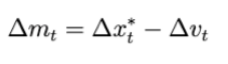
Where:

• ∆mt is the target growth rate of the money supply

• ∆x∗t is the target growth rate of nominal GDP

• ∆vt is the expected change in the velocity of money

Unlike the Taylor Rule, the McCallum Rule does not require estimating the neutral interest rate (r*) or the output gap, instead incorporating principles from the Quantitative Theory of Money (a theory describing the movement of money and its implications for the inflation rate), and is particularly useful in situations where interest rates are near zero and conventional rules may be less effective. Some economists have suggested targeting nominal GDP as a framework to avoid the zero lower bound problem observed in the United States and Japan in the early 2010s.

Conclusion

In conclusion, the Taylor Rule has significant implications for monetary policy frameworks across the world, promoting inflation targeting as an approach for monetary policy implementation rather than nominal GDP targeting.  The systematic approach towards monetary policy has a significant role during periods of economic stability; however, it is clear that more discretionary approaches are required during periods of economic uncertainty or crisis. While the Taylor Rule may not always be followed mechanically, it serves as a guidance for monetary policy frameworks using inflation targeting.